
The backpropagation algorithm has dominated the field of neural network training for a long time. Despite its popularity and effectiveness, it has its disadvantages; in particular, it works differently compared to the human brain.
During the NeurIPS 2022 conference held late last year, Jeffrey Hinton proposed Forward-Forward — a new neural network learning algorithm. His idea was to use it as an alternative to the backpropagation method. FF offers a higher flexibility and uses less memory than backpropagation in architectures with multiple hidden layers. Its main feature is that it is based on contemporary understanding of the workings of human brain.
In this article, we will discuss what contributed to the emergence of this algorithm, how it works, and how to train a simple classification neural network on the MNIST dataset.
Background
The backpropagation algorithm has a number of limitations: it requires saving activations on each layer, which are necessary for calculating the correct derivative. In addition, incoming data cannot be received during the derivative calculation. In contrast, humans are capable of making inferences and keep learning in real time without stopping to calculate an error. Researchers tend to believe that the brain cannot learn using the backpropagation algorithm. But Jeffrey Hinton wants to make it work exactly like the brain. Hinton believes that the backpropagation algorithm poorly mimics the processes that occur in the human brain during learning. Here is his famous quote about this algorithm: “My view is throw it all away and start again. The future depends on some graduate student who’s deeply suspicious of everything I’ve said.” The graduate student has failed to appear, so Jeffrey himself offers his new approach to learning.
How it works
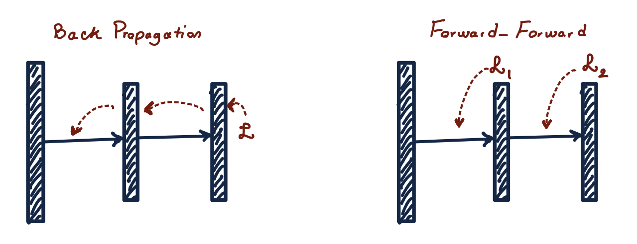
The algorithm is a training procedure for multilayer neural networks inspired by the Boltzmann machine principle. The idea is to replace the standard combination of forward pass and backpropagation algorithm with two forward passes working on different data and having opposite objectives. The positive pass is performed on real data to adjust the weights for increasing goodness in each hidden layer. The negative pass uses artificial data to reduce goodness in each layer. Goodness can be measured in different ways: as the sum of activations squared, or as the negative sum of activations squared.
During the NeurIPS 2022 conference held late last year, Jeffrey Hinton proposed Forward-Forward — a new neural network learning algorithm. His idea was to use it as an alternative to the backpropagation method. FF offers a higher flexibility and uses less memory than backpropagation in architectures with multiple hidden layers. Its main feature is that it is based on contemporary understanding of the workings of human brain.
In this article, we will discuss what contributed to the emergence of this algorithm, how it works, and how to train a simple classification neural network on the MNIST dataset.
Background
The backpropagation algorithm has a number of limitations: it requires saving activations on each layer, which are necessary for calculating the correct derivative. In addition, incoming data cannot be received during the derivative calculation. In contrast, humans are capable of making inferences and keep learning in real time without stopping to calculate an error. Researchers tend to believe that the brain cannot learn using the backpropagation algorithm. But Jeffrey Hinton wants to make it work exactly like the brain. Hinton believes that the backpropagation algorithm poorly mimics the processes that occur in the human brain during learning. Here is his famous quote about this algorithm: “My view is throw it all away and start again. The future depends on some graduate student who’s deeply suspicious of everything I’ve said.” The graduate student has failed to appear, so Jeffrey himself offers his new approach to learning.
How it works
The algorithm is a training procedure for multilayer neural networks inspired by the Boltzmann machine principle. The idea is to replace the standard combination of forward pass and backpropagation algorithm with two forward passes working on different data and having opposite objectives. The positive pass is performed on real data to adjust the weights for increasing goodness in each hidden layer. The negative pass uses artificial data to reduce goodness in each layer. Goodness can be measured in different ways: as the sum of activations squared, or as the negative sum of activations squared.
Let’s imagine that the goodness function for a layer is the sum of the squares of the ReLU activations in that layer. The goal of training is to make goodness much higher than some threshold for real data and lower than the threshold for artificial data.
There is a nuance when training each layer separately. When transferring activations from the first layer to the second layer, determining goodness for the second layer becomes a trivial task, since it can take account of the vector length. There is no need to learn new features to solve this problem, normalization was added to each layer. As a result, the vector length is used in the current layer to determine goodness, and only the direction of this vector remains in the next layer after normalization.
There is a nuance when training each layer separately. When transferring activations from the first layer to the second layer, determining goodness for the second layer becomes a trivial task, since it can take account of the vector length. There is no need to learn new features to solve this problem, normalization was added to each layer. As a result, the vector length is used in the current layer to determine goodness, and only the direction of this vector remains in the next layer after normalization.
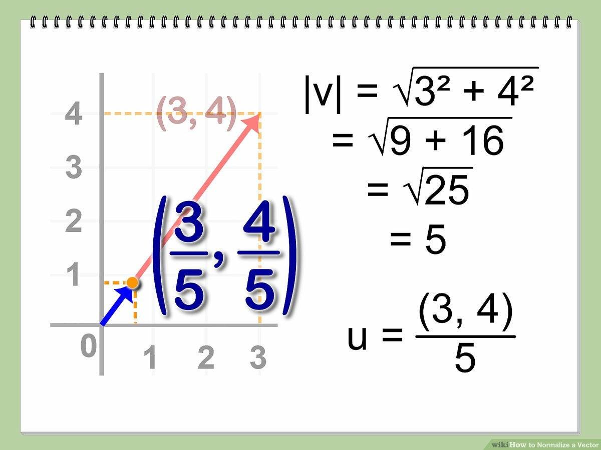
Vector v (red) and its normalized version u (blue).
Training without a training algorithm
We do not need a markup to create vectors representing images, we just need artificial data. This is how we can get a network that clusters similar images and separates different ones in vector space. We can then use trained hidden layers to solve various problems, such as training a linear layer with softmax for image classification. Artificial data can be obtained in many ways. This article deals with the blurring of real images.
Experiments using this approach were successful and showed an error of 1.37% in the neural network with linear layers and 1.16% with convolutional layers.
Training with a training algorithm
Now, let’s consider an example of training a network for classification using the FF algorithm on PyTorch. The notebook is available in the repository https://github.com/Nikita-Sherstnev/forward-forward-algorithm.
Firstly, we import all the necessary libraries and define the device we are going to use for our computations:
import torch
import torch.nn as nn
from tqdm import tqdm
from torch.optim import Adam
from torchvision.datasets import MNIST
from torchvision.transforms import Compose, ToTensor, Normalize, Lambda
from torch.utils.data import DataLoader
import numpy as np

DEVICE = 'cuda'
# DEVICE = 'cpu'
Since we are using a specific function, we cannot simply pass the label as an individual number — it must be included in the input data. So, let’s create a function to add the label to the first (top left) pixels of the image. Since we only have 10 classes available, we need to allocate 10 pixels for this purpose. The labels themselves will appear as one-hot vectors.
def overlay_y_on_x(x, y):
  x_ = x.clone()
  x_[:, :10] *= 0.0
  x_[range(x.shape[0]), y] = x.max()
  return x_
We will also need a function to create negative data — the same images with the wrong labels. So, the label is the only difference between positive and negative instances, and the network will ignore attributes that do not correlate with it. Let’s remove the actual class of the image from the list of all possible classes in the function body so that we do not accidentally get an image with the right class.
def generate_negative_data(x, y):
  y_neg = y.clone()
  for idx, y_samp in enumerate(y):
      allowed_indices = [i for i in range(10)]
      allowed_indices.pop(y_samp.item())
      y_neg[idx] = torch.tensor(np.random.choice(allowed_indices)).to(DEVICE)
  return overlay_y_on_x(x, y_neg)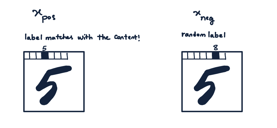
Let’s define the network layer. We use a linear layer as the basis and set the activation function ReLU and the optimizer in the constructor. Here we also define our new hyperparameter — the threshold for separating real and artificial data. This threshold is selected empirically. We need to specify the number of epochs, since each layer is trained separately.
In the forward method, we first calculate the vector length for each instance in the batch and change the shape to enable easy division of the input vectors. This implementation of normalization is what’s described in the article: the average value is not subtracted from the original vectors before division. To avoid division by zero when the vector has zero length, we add a minor epsilon 1e-4 to the divisor. The rest is the same as in the usual linear layer — we multiply the normalized x by the weights, add bias, and use the activation function.
Here, we come to the training method. As a reminder, all layers are trained separately: first, we calculate the goodness function for positive and negative data. In our case it is very simple: pos_loss and neg_loss values should be minimized. Then we combine the resulting tensors and apply the log exp trick to them to prevent the gradient from fading or exploding. After this, we use the average value. We use the backward method to calculate the derivative (in this case, it only calculates the derivative on one layer and does not spread the error over the graph) and make the optimizer step. The algorithm returns the output of the layer which was previously detached from the computation graph. We will need the output as input for the next layer.
class Layer(nn.Linear):
  def __init__(self, in_features, out_features,
               bias=True, device=None, dtype=None):
    super().__init__(in_features, out_features, bias, device, dtype)
    self.relu = torch.nn.ReLU()
    self.opt = Adam(self.parameters(), lr=0.03)
    self.threshold = 3.0
    self.num_epochs = 1000

  def forward(self, x):
    x_direction = x / (x.pow(2).sum(dim=1).sqrt().reshape((x.shape[0], 1)) + 1e-4)

    return self.relu(
             torch.mm(x_direction, self.weight.T) +
             self.bias.unsqueeze(0))

  def train(self, x_pos, x_neg):
    for i in range(self.num_epochs):
      g_pos = self.forward(x_pos).pow(2).mean(1)
      g_neg = self.forward(x_neg).pow(2).mean(1)

      pos_loss = -g_pos + self.threshold
      neg_loss = g_neg - self.threshold

      loss = torch.log(1 + torch.exp(torch.cat([
                                 pos_loss,
                                 neg_loss]))).mean()

      self.opt.zero_grad()

      loss.backward()
      self.opt.step()

      return self.forward(x_pos).detach(), self.forward(x_neg).detach()
Now, let’s define the model. The training method is very simple — we train the layers one by one and pass the result to the next layer. An unusual method is used with inference — calculating the goodness metric for each combination of input data and possible classes, and then returning the class with the highest goodness. You can also use softmax, but the classification results will be less accurate.
class Net(torch.nn.Module):
  def __init__(self, dims):
    super().__init__()
    self.layers = []
    for d in range(len(dims) - 1):
      self.layers += [Layer(dims[d], dims[d + 1]).to(DEVICE)]

  def predict(self, x):
    goodness_per_label = []
    for label in range(10):
      h = overlay_y_on_x(x, label)
      goodness = []

    for layer in self.layers:
      h = layer(h)
      goodness += [h.pow(2).mean(1)]
      goodness_per_label += [sum(goodness).unsqueeze(1)]
    goodness_per_label = torch.cat(goodness_per_label, 1)
    return goodness_per_label.argmax(1)

  def train(self, x_pos, x_neg):
    h_pos, h_neg = x_pos, x_neg
    for i, layer in enumerate(self.layers):
      h_pos, h_neg = layer.train(h_pos, h_neg)
And, finally, we can begin training. Let’s load our dataset, create a three-layer network and start training. We use the previously defined functions to form the input data.
torch.manual_seed(1234)
train_loader, test_loader = MNIST_loaders()

net = Net([784, 512, 512])

for x, y in tqdm(train_loader):
  x, y = x.to(DEVICE), y.to(DEVICE)

  x_pos = overlay_y_on_x(x, y)
  x_neg = generate_negative_data(x, y)

  net.train(x_pos, x_neg)
With this configuration, the error was 2.04% on the training data and 4.74% on the test data. The neural network trained for this article showed an error of 0.64%, but the author trained the network with 4 hidden layers of 2000 neurons each on augmented data. In addition, the author did not use the first hidden layer when calculating the goodness metric. This configuration only made my results worse: the error reached 11%, so it was not possible to reproduce the results of the article. Training with augmentation was not tested. You can experiment with the code and see what happens.
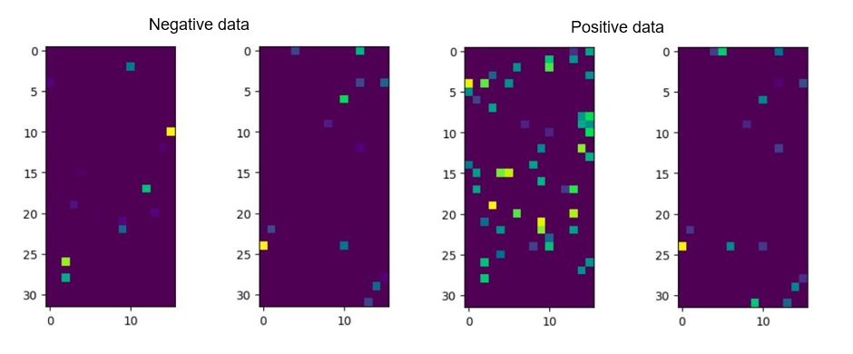
If we visualize activations in the hidden layers, we will see that the “neuron” activity is higher on positive data than on negative data. In this case, our network input was an image of the number seven with the labels 0 and 7.
If we visualize activations in the hidden layers, we will see that the “neuron” activity is higher on positive data than on negative data. In this case, our network input was an image of the number seven with the labels 0 and 7.
Jeffrey also conducted an experiment on the CIFAR-10 dataset in his article. When using backpropagation, the error decreased much faster, and accuracy was slightly lower with FF.
FF as an alternative to GAN
GAN (generative adversarial network) uses a multilayer network to generate data and trains its generative model with a multilayer discriminative network to distinguish the generated data from the real data. In practice, GANs generate quite realistic images, but they are prone to so-called mode collapse: there may be an image space in which they generate nothing. In addition, they are trained by the backpropagation algorithm, so it is difficult to imagine them operating in the cerebral cortex.
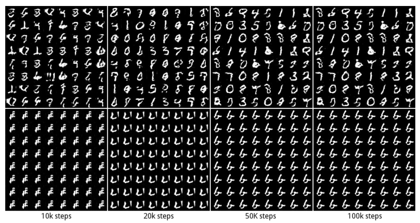
Mode collapse example: the generator hits the local minimum and generates the same images
FF can be seen as a special case of GAN in which each layer of the discriminative model makes its own decision about the data plausibility, and there is no need for backpropagation. There is also no need to use backprop to train a generative network because it can overuse the discriminative model weights. The only thing the model has to learn is how to convert hidden representations into generated data. There is no need for backpropagation when using linear transformation to calculate softmax logits. This approach will help prevent mode collapse and the issue when one model needs less training time than the other.
Sleep
The Forward-Forward algorithm would be much easier to imagine, if positive data were processed while awake, and negative data were generated by the neural network and processed in sleep.
Using the sum of activation squares as the goodness function, alternating between thousands of updates of weights on real data and thousands of updates on artificial data only works with very low learning rate and very high momentum. It is possible that another goodness function would allow us to separate the positive phase from the negative phase, and this is probably the most important question about the FF algorithm as a biological model.
When separating the positive and negative phases, it would be interesting to see how the suspension of training on artificial data results in an effect similar to serious sleep deprivation.
Mortal computing
In terms of energy costs, an efficient way to multiply activations by a matrix of weights is to implement activations as voltages and weights — as conductors. Their product is the charges that accumulate over time. This seems more reasonable than using transistors with high power consumption to simulate individual bits in the binary representation of a number and performing O(n^2) bitwise operations to multiply two n-bit numbers. Unfortunately, it is difficult to implement the backpropagation algorithm so effectively.
Modern computers were designed to follow instructions unconditionally and with a clear distinction between software and hardware, so that a program written on one computer could be transferred to another. This makes the program immortal: knowledge does not die when the hardware dies. The separation of software from hardware is one of the fundamental principles of Computer Science, which offers many advantages. You can study a program without going into the details of electrical engineering, or you can write a program and copy it on to a million computers. Or you can compute derivatives on a large dataset using several copies of the model running in parallel. You can save on electricity and computer manufacturing if you are willing to give up immortality. In the future, we may need to train new computers for specific tasks. Since the parameters trained on such computers cannot be directly copied to other machines, the computations are mortal and tied to the hardware.
According to Hinton, if one wants to achieve energy-efficient neural network computation, he should use mortal computing. Such computations are only possible with a training algorithm that can run efficiently on hardware whose exact configuration is unknown. Forward-Forward is a promising candidate in this case, although it remains to be seen how it will perform in large architectures.
Development paths
Research on the Forward-Forward (FF) algorithmis still in its early stages, and many questions remain open:
● Can FF reproduce a generative model of images or videos that are good enough to generate negative data for training without a training algorithm?
● What is the best goodness function to use? Based on the latest results, minimizing the sum of activities without squaring them also works well.
● What is the best activation function to use? So far, only ReLU has been analyzed.
● In terms of spatial data, can FF benefit from multiple goodness functions computed from individual image areas?
● In terms of serial data, can fast weights be used to mimic a simplified transformer?
The official implementation of the algorithm is not yet in the public domain. Hinton wrote his code in MATLAB and does not want to share it with the general public. In 1986, Hinton published an article with his colleagues on the use of backprop in neural network training. Everyone was rather skeptical about this algorithm until the advent of GPUs with the ability to be trained on large datasets. Perhaps FF’s finest hour will come much sooner.
Now you know how the Forward-Forward algorithm works, what advantages and disadvantages it has, and how it simulates the behavior of real neurons in the brain. If you are passionate about research, we are sure you will want to get to the bottom of this hot topic and modify the algorithm to solve your tasks.